NOTE: Article in Progress
From data to insights
1. Lifecycle of data
Lifecycle of data: data, knowledge, insights, action
Data to knowledge
- Data acquisition
- Data Extraction
- Data Cleaning
- Data Transformation
- ETL
- Data analysis modeling
- Data Storage
- Analysis
- Visualisation

Knowledge to Insights
Knowledge to Knowledge
Insights to Action
Insights to Knowledge
Action to Data
Data analysis
Data visualisation
finding known and unknown patterns from data
ETL (Extraction Transformation and Loading)
- Data Extraction
- Data Cleaning
- Data Transformation
- Loading data to information stores
2. Data Acquistion and Storage
2.1. Data acquisition



- Surveys
- Manual surveys
- Online surveys
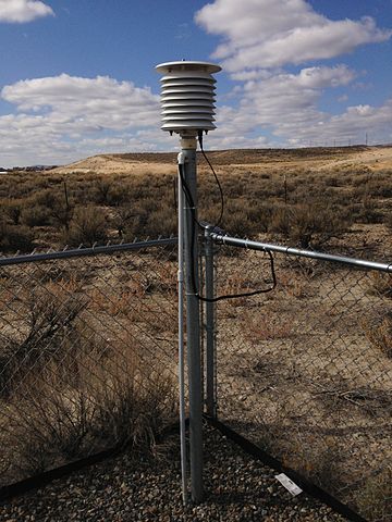
- Sensors1
- Temperature, pressure, humidity, rainfall
- Acoustic, navigation
- Proximity, presence sensors
- Social networks
- Video surveillance cameras
- Web
2.2. Data storage formats
- Binary and Textual Files
- CSV/TSV
- XML
- JSON
- Media (Images/Audio/Video)
2.3 Types of data stores
- Structured data stores
- Relational databases
- Object-oriented databases
- Unstructured data stores
- Filesystems
- Content-management systems
- Document collections
- Semi-structured data stores
- Filesystems
- NoSQL data stores

NoSQL versus SQL5: no strict schemas and no horizontal scaling for NoSQL data stores.
2.3.1. ACID Transactions1
- Atomicity: Each transaction must be "all or nothing".
- Consistency: Any transaction must bring database from one valid state to another.
- Isolation: Both concurrent execution and sequential execution of transactions must bring the database to same state.
- Durability: Irrespective of power losses, crashes, a transaction once committed to the database must remain in that state.
- https://en.wikipedia.org/wiki/ACID
- Ensure validity of databases even in case of errors, power failures
- Important in banking sector
2.3.2. Types of data stores
- Relational databases
- Object-oriented databases
- NoSQL (Not only SQL) data stores
- NewSQL
2.3.3. NoSQL
- Comprises consistency
- Focus on availability and speed
2.3.4. Types of NoSQL stores
- Column-oriented database
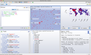
- Document-oriented database
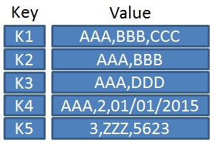
- Key-value database
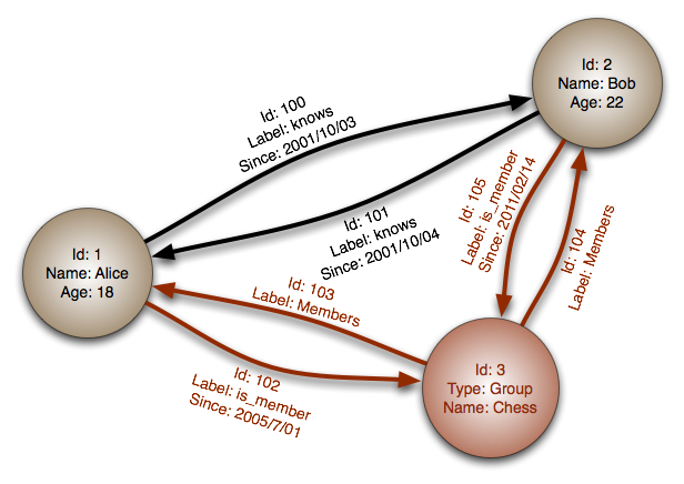
- Graph-oriented database
.png)
3. Data Extraction and Integration
3.1. Data extraction techniques
- Data dumps
- Downloading complete data dumps
- Downloading selective data dumps
- Periodical polling of data feeds (e.g., blogs, news feeds)
- Data streams
- Subscrbing to data streams (push notifications)
3.2. Query interfaces
- Query endpoints supporting declarative languages
- SQL
- SPARQL
- Automated Manual search (and filter) options
3.3. Crawlers for web pages

3.4. Application Programming Interface (API)
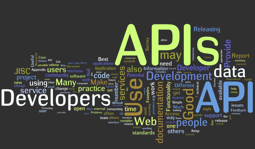
- Web operations (CRUD) to manipulate externally managed resources
- Requires programmers to develop wrappers for web service integration
4. Pre-treatement of Data
4.1 Data Cleaning: Types of Errors
- Syntactical errors
- Semantical errors
- Data coverage errors
4.1.1. Syntactical errors
- Lexical errors (e.g., user entered a string instead of a number)
- Data format errors (e.g, order of last name, first name)
- Irregular data errors (e.g., usage of different metrics)
4.1.2. Semantic errors
- Violation of integrity constraints
- Contradiction
- Duplication
- Invalid data (unable to detect despite presence of triggers and integrity constraints)
4.1.3. Coverage errors
- Missing values
- Missing data
4.2. Data Cleaning: Handling Errors
4.2.1. Handling Syntactical errors
- Validation using schema (e.g., XSD, JSONP)
- Data transformation
4.2.2. Handling Semantic errors
- Duplicate elimination using techniques like specifying integrity constraints like functional dependencies
4.2.3. Handling Coverage errors
- Interpolation techniques
- External data sources
4.2.4. Administrators and handling errors
- User feedback
- Alerts and triggers
5. Data Transformation
Languages
- Template languages
- XSLT
- AWK
- Sed
- Programming languages like PERL
6. ETL
6.1. ETL (Extraction Transformation and Loading)
- Data Extraction
- Data Cleaning
- Data Transformation
- Loading data to information stores

6.2.1. Models for data analysis
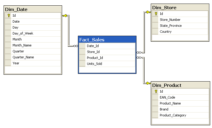
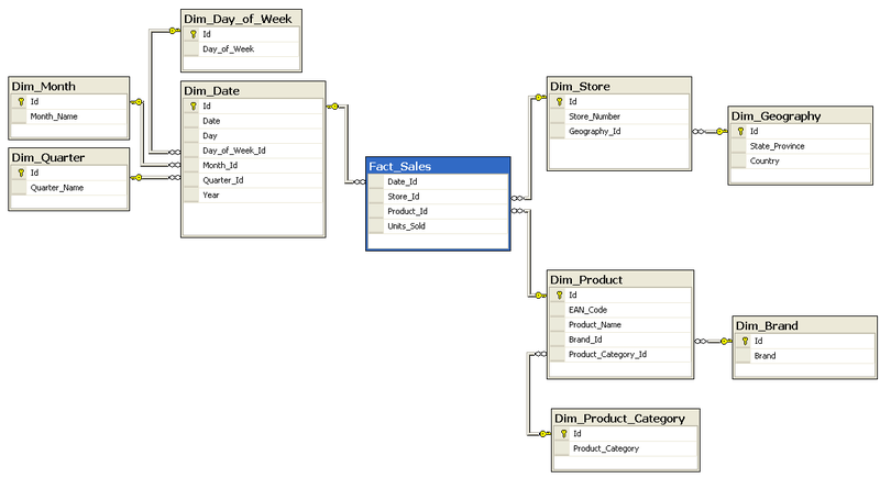
- Multidimensional data analysis
- Dimensions
- Attributes
- Levels
- Hierarchies
- Facts
- Measures
- Multidimensional data analysis: Examples
- Dimensions (e.g.Spatio-temporal dimensions, Product)
- Attributes (e.g. Name, Manufactures etc.)
- Levels (e.g., Day, Month, Quarter, Store, City, Country etc.)
- Hierarchies (e.g., Day-Month-Quarter-Year, Store-City-Country etc.)
- Facts
- Measures (e.g., Number of products sold/unsold)
6.2.2. Star Schema
6.2.3. Data Cubes
- Data cubes for online analytical processing (OLAP)
- OLAP Cube operations
- Slice
- Dice
- Drill up/down
- Pivot
6.2.4. Snow Schema
6.2. ETL: From one data store to another
- From: Data sources
- Internal or external databases
- Web Services
- To: Data warehouses
- Enterprise warehouses
- Web warehouses
7. Data Analysis
Activities of data analysis
- Retrieving values
- Filter
- Compute derived values
- Find extremum
- Sort
- Determine range
- Characterize distribution
- Find analysis
- Cluster
- Correlate
- Contextualization
8. Data Visualization
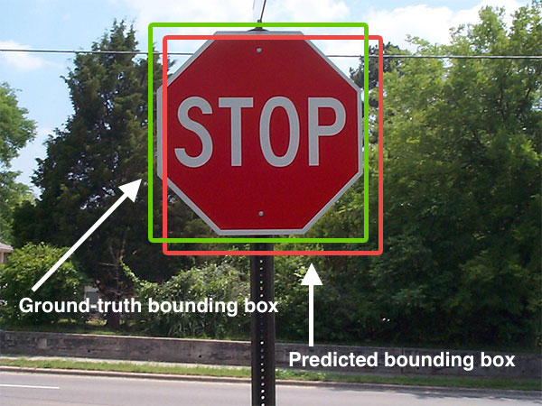
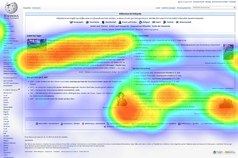
8.1. Types of Data Visualization
- Time-series
- Ranking
- Part-to-whole
- Deviation
- Sort
- Frequency distribution
- Correlation
- Nominal comparison
- Geographic or geospatial
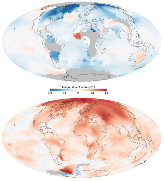
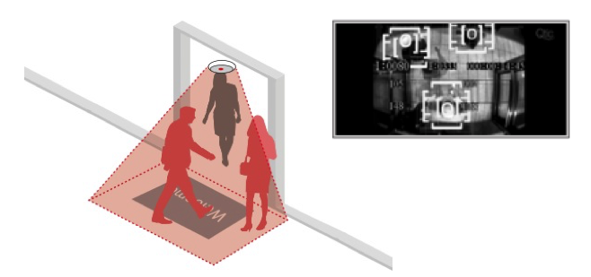
8.2. Data Visualization: Examples
- Bar-chart (Nominal comparison)
- Pie-chart (part-to-whole)
- Histograms (frequency-distribution)
- Scatter-plot (correlation)
- Network
- Line-chart (time-series)
- Treemap
- Gantt chart
- Heatmap
Pie Chart


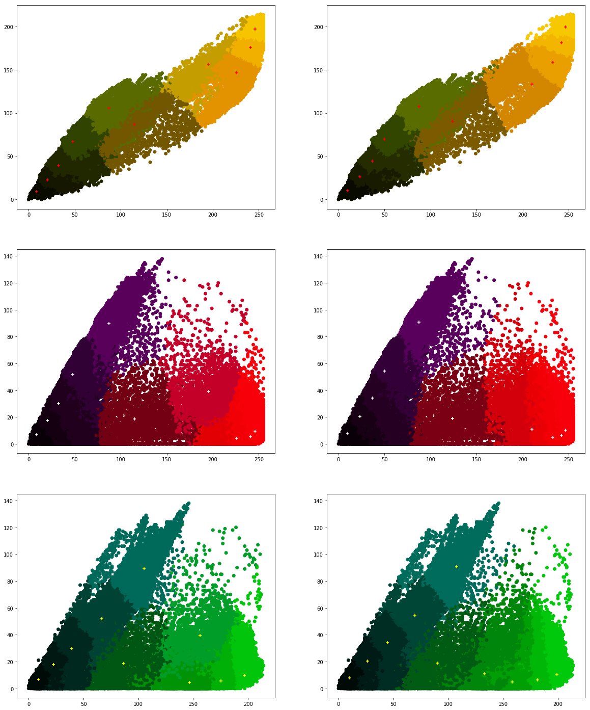
k Predominant colours

RGB Scatter plots (Comparison)

9. Patterns


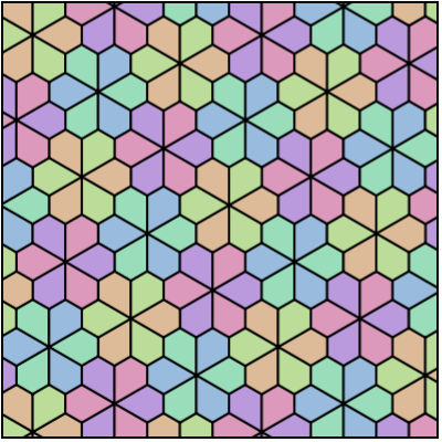
9.1. Patterns in Nature


.jpg)
- Symmetry
- Trees, Fractals
- Spirals
- Chaos
- Waves
- Bubbles, Foam
- Tesselations
- Cracks
- Spots, stripes
9.2. Patterns by Humans
- Buildings (Symmetry)
- Cities
- Virtual environments (e.g., video games)
- Human artifacts

Pattern creation
- Repitition
- Fractals
- Julia set: f(z) = z2 + c

.png)
Synonyms
- Pattern recognition
- Knowledge discovery in databases
- Data mining2
- Machine learning
Data mining trends2 future (2007)3 finding patterns in data4
Pattern Recognition
- Goal is to detect patterns and regularities in data
- Approaches
- Supervised learning: Availability of labeled training data
- Unsupervised learning: No labeled training data available
- Semi-supervised learning: Small set of labeled training data and a large amount of unlabeled data
- Self-supervised learning: automated generation of labels for training
Formalization
- Euclidean vector: geometric object with magnitude and direction
- Vector space: collection of vectors that can be added together and multiplied by numbers.
- Feature vector: n-dimensional vector
- Feature space: Vector space associated with the vectors
Examples: Features
- Images: pixel values.
- Texts: Frequency of occurence of textual phrases.
Formalization
- Feature construction1: construction of new features from already available features
- Feature construction operators
- Equality operators, arithmetic operators, array operators (min, max, average etc.)...
Example
- Let Year of Birth and Year of Death be two existing features.
- A new feature called Age = Year of Birth - Year of Death
- https://en.wikipedia.org/wiki/Feature_vector
Formalization: Supervised learning
- Let N be the number of training examples
- Let X be the input feature space
- Let Y be the output feature space (of labels)
- Let {(x1, y1),...,(xN, yN)} be the N training examples, where
- xi is the feature vector of ith training example.
- yi is its label.
- The goal of supervised learning algorithm is to find g: X → Y, where
- g is one of the functions from the set of possible functions G (hypotheses space)
- Scoring function F denote the space of scoring functions, where
- f: X × Y → R such that g returns the highest scoring function.
Formalization: Unsupervised learning
- Let X be the input feature space
- Let Y be the output feature space (of labels)
- The goal of unsupervised learning algorithm is to
- find mapping X → Y
Formalization: Semi-supervised learning
- Let X be the input feature space
- Let Y be the output feature space (of labels)
- Let {(x1, y1),...,(xl, yl)} be the l be the set of labeled training examples
- Let {xl+1,...,xl+u} be the u be the set of unlabeled feature vectors of X.
- The goal of semi-supervised learning algorithm is to do
- Transductive learning, i.e., find correct labels for {xl+1,...,xl+u}. OR
- Inductive learning, i.e., find correct mapping X → Y
10. Data Mining
Tasks in Data Mining
- Classification
- Clustering
- Regression
- Sequence Labeling
- Association Rules
- Anomaly Detection
- Summarization
10.1. Classification
- Generalizing known structure to apply to new data
- Identifying the set of categories to which an object belongs
- Binary vs. Multiclass classification
Applications
- Spam vs Non-spam
- Document classification
- Handwriting recognition
- Speech Recognition
- Internet Search Engines
Formal definition
- Let X be the input feature space
- Let Y be the output feature space (of labels)
- The goal of classification algorithm (or classifier) is to find {
(x1, y1),...,(xl, yk)}, i.e., assigning a known label to every input feature vector, where
- xi ∈ X
- yi ∈ Y
- |X | = l
- |Y | = k
- l >= k
Classifiers
- Classifying Algorithm
- Two types of classifiers:
- Binary classifiers assigning an object to any of two classes
- Multiclass classifiers assigning an object to one of several classes
Linear Classifiers
- A linear function assigning a score to each possible category by combining the feature vector of an instance with a vector of weights, using a dot product.
- Formalization:
- Let X be the input feature space and xi ∈ X
- Let βk be vector of weights for category k
- score(xi, k) = xi.βk, score for assigning category k to instance xi. The category that gives the highest score is assigned as the category of the instance.
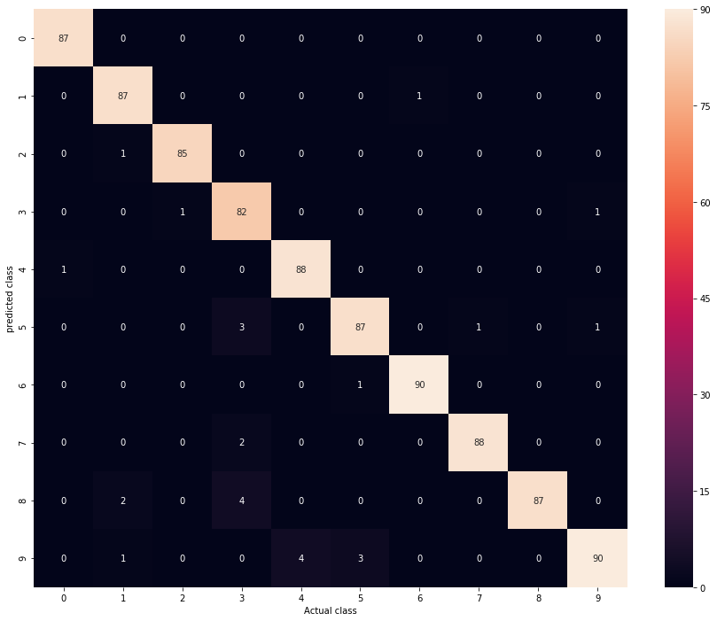
Classifiers
Let
- tp: number of true postives
- fp: number of false postives
- fn: number of false negatives
Then
- Precision p = tp / (tp + fp)
- Recall r = tp / (tp + fn)
- F1-score f1 = 2 * ((p * r) / (p + r))
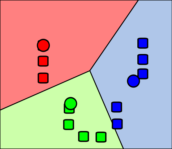
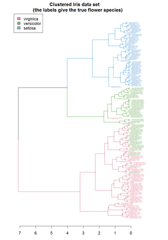
10.2. Clustering
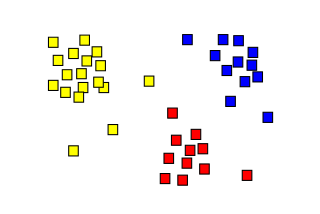
- Discovering groups and structures in the data without using known structures in the data
- Objects in a cluster are more similar to each other than the objects in the other cluster
Applications
- Social network analysis
- Image segmentation
- Recommender systems
- Grouping of shopping items
Formal definition
- Let X be the input feature space
- The goal of clustering is to find k subsets of X, in such a way that
- C1.. ∪ ..Ck ∪ Coutliers = X and
- Ci ∩ Cj = ϕ, i ≠ j; 1 <i,j <k
- Coutliers may consist of outlier instances (data anomaly)
Cluster models
- Centroid models: cluster represented by a single mean vector
- Connectivity models: distance connectivity
- Distribution models: clusters modeled using statistical distributions
- Density models: clusters as connected dense regions in the data space
- Subspace models
- Group models
- Graph-based models
- Neural models
10.3. Regression
- Finding a function which models the data
- Assigns a real-valued output to each input
- Estimating the relationships among variables
- Relationship between a dependent variable ('criterion variable') and one or more independent variables ('predictors').

Applications
- Prediction
- Forecasting
- Machine learning
- Finance
Formal definition
- A function that maps a data item to a prediction variable
- Let X be the independent variables
- Let Y be the dependent variables
- Let β be the unknown parameters (scalar or vector)
- The goal of regression model is to approximate Y with X,β, i.e.,
- Y ≅ f(X,β)
Linear regression
- straight line: yi = β0 + β1xi + εi OR
- parabola: yi = β0 + β1xi + β1xi2 +εi
Linear regression
- straight line: yi = β0 + β1xi + εi OR
- ŷi = β0 + β1i OR
- Residual: ei = ŷi - yi
- Sum of squared residuals, SSE = Σ ei, where 1 < i < n
- The goal is to minimize SSE
10.4. Sequence Labeling
- Assigning a class to each member of a sequence of values
Applications
- Part of speech tagging
- Linguistic translation
- Video analysis
- Handwriting recognition
- Information extraction
Formal definition
- Let X be the input feature space
- Let Y be the output feature space (of labels)
- Let 〈x1,...,xT〉 be a sequence of length T.
- The goal of sequence labeling is to generate a corresponding sequnce
- 〈y1,...,yT〉 of labels
- xi ∈ X
- yj ∈ Y
10.5. Association Rules
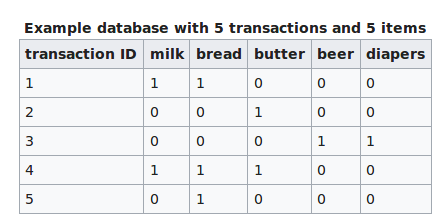
Association Rules
- Searches for relationships between variables
Applications
- Web usage mining
- Intrusion detection
- Affinity analysis
Formal definition
- Let I be a set of n binary attributes called items
- Let T be a set of m transactions called database
- Let I = {(i1,...,in)} and T = {(t1,...,tm)}
- The goal of association rule learning is to find
- X ⇒ Y, where X ⇒ Y ⊆ I
- X is the antecedent
- Y is the consequent
Formal definition
- Support: how frequently an itemset appears in the database
- supp(X) = |t ∈T; X ⊆ t| / |T|
- Confidence: how frequently the rule has been found to be true.
- conf(X ⇒ Y) = supp(X ∪ Y)/supp(X)
- Lift: the ratio of the observed support to that of the expected if X and Y were independent
- lift(X ⇒ Y) = supp(X ∪ Y)/(supp(X) ⨉ supp(Y))
Example
- {bread, butter} ⇒ {milk}
10.6. Anomaly Detection
- Identification of unusual data records
- Approaches
- Unsupervised anomaly detection
- Supervised anomaly detection
- Semi-supervised anomaly detection
Applications
- Intrusion detection
- Fraud detection
- Remove anomalous data
- System health monitoring
- Event detection in sensor networks
- Misuse detection
Characteristics
- Unexpected bursts
Formalization
- Let Y be a set of measurements
- Let PY(y) be a statistical model for the distribution of Y under 'normal' conditions.
- Let T be a user-defined threshold.
- A measurement x is an outlier if PY(x) < T
10.7. Summarization
- Providing a more compact representation of the data set
- Report Generation
Applications
- Keyphrase extraction
- Document summarization
- Search engines
- Image summarization
- Video summarization: Finding important events from videos
Formalization: Multidocument summarization
- Let {D = D1, ..., Dk} be a document collection of k documents
- A Document {D = t1, ..., tm} consists of m textual units (words, sentences, paragraphs etc.)
- Let {D = t1, ..., tn} be the complete set of all textual units from all documents, where
- ti ∈ D, if and only if ∃ Dj such that ti ∈ Dj
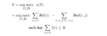
- S ⊆ D constitutes a summary
- Two scoring functions
- Rel(i): relevance of textual unit i in the summary
- Red(i,j): Redundancy between two textual units ti, tj
- Scoring for a summary S
- s(S) score of summary S
- l(i) is the length of the textual unit i
- K is the fixed maximum length of the summary
- Finding a subset from the entire subset
- Approaches
- Extraction: Selecting a subset of existing words, phrases, or sentences in the original text without any modification
- Abstraction: Build an internal semantic representation and then use natural language generation techniques
Extractive summarization
- Approaches
- Generic summarization: Obtaining a generic summary
- Query relevant summarization: Summary relevant to a query
11. Algorithms
- Support Vector Machines (SVM)
- Stochastic Gradient Descent (SGD)
- Nearest-Neighbours
- Naive Bayes
- Decision Trees
- Ensemble Methods (Random Forest)
11.1. Support Vector Machines (SVM)
Introduction
- Supervised learning approach
- Binary classification algorithm
- Constructs a hyperplane ensuring the maximum separation between two classes

Hyperplane
- Hyperplane of n-dimensional space is a subspace of dimension n-1
- Examples
- Hyperplane of a 2-dimensional space is 1-dimensional line
- Hyperplane of a 3-dimensional space is 2-dimensional plane
Formal definition
- The goal of a SVM is to estimate a function f: RN ⨉ {+1,-1}, i.e.,
- If x1,...,xl ∈ RN are the N input data points,
- the goal is to find (x1,y1),...,(xl,yl) ∈ RN ⨉ {+1,-1}
- Any hyperplane can be written by the equation using set of input points x
- w.x - b = 0, where
- w ∈ RN, a normal vector to the plane
- b ∈ R
- A decision function is given by f(x) = sign(w.x - b )

Formal definition
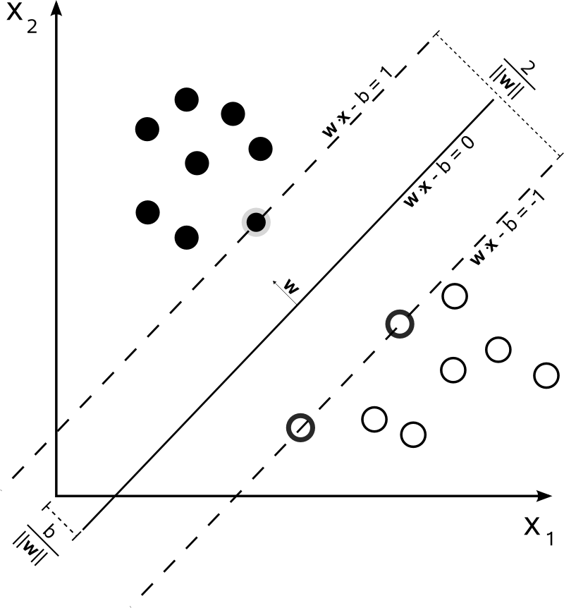
- If the training data are linearly separable, two hyperplanes can be selected
- They separate the two classes of data, so that distance between them is as large as possible.
- The hyperplanes can be given by the equations
- w.x - b = 1
- w.x - b = -1
- The distance between the two hyperplanes can be given by 2/||w||
- Region between these two hyperplanes is called margin.
- Maximum-margin hyperplane is the hyperplane that lies halfway between them.
Formal definition
- In order to prevent data points from falling into the margin, following constraints are added
- w.xi - b >= 1, if yi = 1
- w.xi - b <= -1, if yi = -1
- yi(w.xi - b) >= 1 for 1<= i <= n
- The goal is to minimize ||w|| subject to yi(w.xi - b) >= 1 for 1<= i <= n
- Solving for both w and b gives our classifier f(x) = sign(w.x - b)
- Max-margin hyperplane is completely determined by the points that lie nearest to it, called the support vectors
Data mining tasks
- Classification (Multi-class classification)
- Regression
- Anomaly detection
Applications
- Text and hypertext categorization
- Image classification
- Handwriting recognition
11.2. Stochastic Gradient Descent (SGD)
- A stochastic approximation of the gradient descent optimization
- Iterative method for minimizing an objective function that is written as a sum of differentiable functions.
- Finds minima or maxima by iteration
Gradient
- Multi-variable generalization of the derivative.
- Gives slope of the tangent of the graph of a function
- Gradient points in the direction of the greatest rate of increase of a function
- Magnitude of gradient is the slope of the graph in that direction

Gradient vs Derivative
- Derivatives defined on functions of single variable
- Gradient defined on functions of multiple variables
- Gradient is a vector-valued function (range is a vector)
- Derivative is a scalar-valued function

Gradient descent
- First-order iterative optimization algorithm for finding the minimum of a function.
- Finding a local minima involves taking steps proportional to the negative of the gradient of the function at the current point.

Standard gradient descent method
- Let's take the problem of minimizing an objective function
- Q(w) = 1/n (ΣQi(w)), 1<=i<n
- Summand function Qi associated with ith observation in the data set.
- w = w - η.∇ Q(w)
Iterative method
- Choose an initial vector of parameters w and learning rate η.
- Repeat until an approximate minimum is obtained:
- Randomly shuffle examples in the training set.
- w = w - η.∇ Qi(w), for i=1...n
Applications
- Classification
- Regression
11.3. Nearest-Neighbours
k-nearest neighbors algorithm
- k-NN classification: output is a class membership
(object is classified by a majority vote of its neighbors.) - k-NN regression: output is the property value for the object (average values of its k nearest neighbors)

Applications
- Regression
- Anomaly detection
11.4. Naive Bayes classifiers
- Collection of simple probabilistic classifiers based on applying Bayes' theorem with strong independence assumption between the features.
Applications
- Document classification (spam/non-spam)
Bayes' Theorem
- If A and B are events.
- P(A), P(B) are probabilities of observing A and B independently of each other..
- P(A|B) is conditional probability, the likelihood of event A occurring given that B is true
- P(B|A) is conditional probability, the likelihood of event B occurring given that A is true
- P(B) ≠ 0
- P(A|B) = (P(B|A).P(A))/P(B)
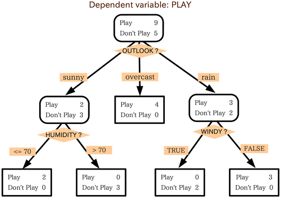
11.5. Decision Trees
- Decision support tool
- Tree-like model of decisions and their possible consequences
Applications
- Classification
- Regression
- Decision Analysis: identifying strategies to reach a goal
- Operations Research
11.6. Ensemble Methods (Random Forest)
Defintion
- Collection of multiple learning algorithms to obtain better predictive performance than could be obtained from one of the constituting algorithms alone.
- Random forests are obtained by building multiple decision trees at training time
- Multiclass classification
- Multilabel classification (the problem of assigning one or more label to each instance. There is no limit on the number of classes an instance can be assigned to.)
- Regression
- Anomaly detection
12. Feature Selection
Definition
- Process of selecting a subset of relevant features
- Used in domains with large number of features and comparatively few sample points
Applications
- Analysis of written texts
- Analysis of DNA microarray data
Formal defintion[8]
- Let X be the original set of n features, i.e., |X| = n
- Let wi be the weight assigned to feature xi∈ X
- Binary feature selection assigns binary weights whereas continuous feature selection assigns weights preserving the order of its relevance.
- Let J(X') be an evaluation measure, defined as J: X' ⊆ X → R
- Feature selection problem may be defined in three following ways
- |X'| = m < n. Find X' ⊂ X such that J(X') is maximum
- Choose J0, Find X' ⊆ X, such that J(X') >= J0
- Find a compromise among minimizing |X'| and maximizing J(X')
Data Mining
Goals
- Artifical Neural Networks
- Deep Learning
- Reinforcement Learning
- Data Licences, Ethics and Privacy
13. Artificial Neural Networks
- Inspired by biological neural networks
- Collection of connected nodes called artificial neurons.
- Artificial neurons can transmit signal from one to another (like in a synapse).
- Signal between artificial neurons is a real number
- The output of a neuron is the sum of weighted inputs.

Perceptron
- Algorithm for supervised learning of binary classifiers
- Binary classifier

Perceptron: Formal definition
- Let y = f(z) be output of perceptron for an input vector z
- Let N be the number of training examples
- Let X be the input feature space
- Let {(x1, d1),...,(xN, dN)} be the N training examples, where
- xi is the feature vector of ith training example.
- di is the desired output value.
- xj,i be the ith feature of jth training example.
- xj,0 = 1
- Weights are represented in the following manner:
- wi is the ith value of weight vector.
- wi(t) is the ith value of weight vector at a given time t.
Perceptron: Steps
- Initialize weights and threshold
- For each example (xj, dj) in training set
- Calculate the weight: yj(t)=f[w(t).xj]
- Update the weights: wi(t + 1) = wi(t) + (dj-yj(t))xj,i
- Repeat step 2 until the iteration error 1/s (Σ |dj - yj(t)|) is less than user-specified threshold.
Backpropagation
- Backward propagation of errors
- Adjust the weight of neurons by calculating the gradient of the loss function
- Error is calculated and propagated back to the network layers
14. Deep Learning
Deep neural networks
- Multiple hidden layers between the input and output layers
Applications
- Computer vision
- Speech recognition
- Drug design
- Natural language processing
- Machine translation
Convolutional deep neural networks
- Analysis of images
- Inspired by neurons in the virtual cortex
- Network learns the filters

15. Reinforcement Learning
- Inspired by behaviourist psychology
- Actions to be taken in order to maximize the cumulative award.

16. Data Licences, Ethics and Privacy
- Data usage licences
- Confidentiality and Privacy
- Ethics

Big Data
- Volume
- Variety
- Velocity
- Veracity
- Value


References
- Data Mining course by John Samuel (2017)
- Piatetsky-Shapiro, Gregory. “Data Mining and Knowledge Discovery 1996 to 2005: Overcoming the Hype and Moving from ‘University’ to ‘Business’ and ‘Analytics.’” Data Mining and Knowledge Discovery, vol. 15, no. 1, July 2007, pp. 99–105. DOI.org (Crossref), doi:10.1007/s10618-006-0058-2.
- Kriegel, Hans-Peter, et al. “Future Trends in Data Mining.” Data Mining and Knowledge Discovery, vol. 15, no. 1, July 2007, pp. 87–97. DOI.org (Crossref), doi:10.1007/s10618-007-0067-9.
- Fayyad, Usama, et al. “Knowledge Discovery and Data Mining: Towards a Unifying Framework.” Proceedings of the Second International Conference on Knowledge Discovery and Data Mining, AAAI Press, 1996, pp. 82–88.
- NoSQL vs. SQL